Traditional image classification models, such as Convolutional Neural Networks (CNNs) (opens new window), have been the cornerstone of computer vision (opens new window) tasks for years. These models operate by training on large, labeled datasets where each image is associated with a specific class label. Typically, these models rely on N-shot learning, meaning they require a large number of labeled images (N examples) for each class to achieve high accuracy.
However, these traditional models come with several significant challenges. First, they demand a substantial amount of labeled data, which is time-consuming and costly to produce. Additionally, traditional models struggle to generalize effectively, especially when the number of examples (N) is small.
Moreover, these models are limited in their ability to classify unseen data. If a model hasn’t been trained on a specific class, it is unlikely to accurately classify images from that class. This limitation becomes a significant bottleneck, especially in scenarios where new categories frequently emerge or where labeled data is scarce.
These challenges make it clear that we need smarter models that can do more with less. That’s where CLIP really shines. Unlike traditional models, CLIP doesn’t need to be specifically trained in every class to recognize it. It uses a huge dataset of image-text pairs and contrastive learning to figure out what’s in an image, even if it hasn’t seen that type of image before. This makes CLIP incredibly useful, especially in situations where traditional models fall short.
# CLIP
OpenAI launched CLIP (opens new window) in 2021, a model that bridges the gap between images and text by placing them in a shared vector space. By using contrastive learning, CLIP learns to tell which image-text pairs belong together and which don't. This ability lets it generalize across different classes, even those it hasn’t encountered before. As a result, CLIP is highly effective at zero-shot classification, where it can accurately identify new categories based purely on text descriptions.
- Zero-Shot Classification (opens new window): This approach lets the model classify new categories without needing any labeled examples during training. It’s called "zero-shot" because it requires zero training data, relying only on text descriptions to make predictions.
- N-Shot Classification (opens new window): In this case, the model requires N labeled examples per category to learn how to classify them correctly. The "N" represents the number of examples the model needs to see to understand each category.
# How CLIP is used for Zero-Shot Classification
CLIP’s architecture is designed to handle zero-shot classification in a straightforward yet powerful way. At the core of CLIP are two encoders: one for images and one for text. These encoders transform input images and text descriptions into high-dimensional vectors, or embeddings, within a shared vector space.
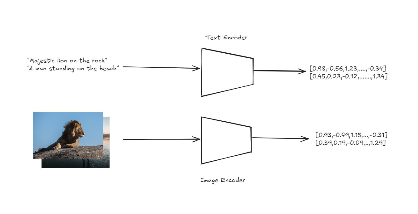
Text and Image encoders to get embeddings
The key innovation here is that both images and text are represented in the same space, enabling direct comparison between the two modalities.
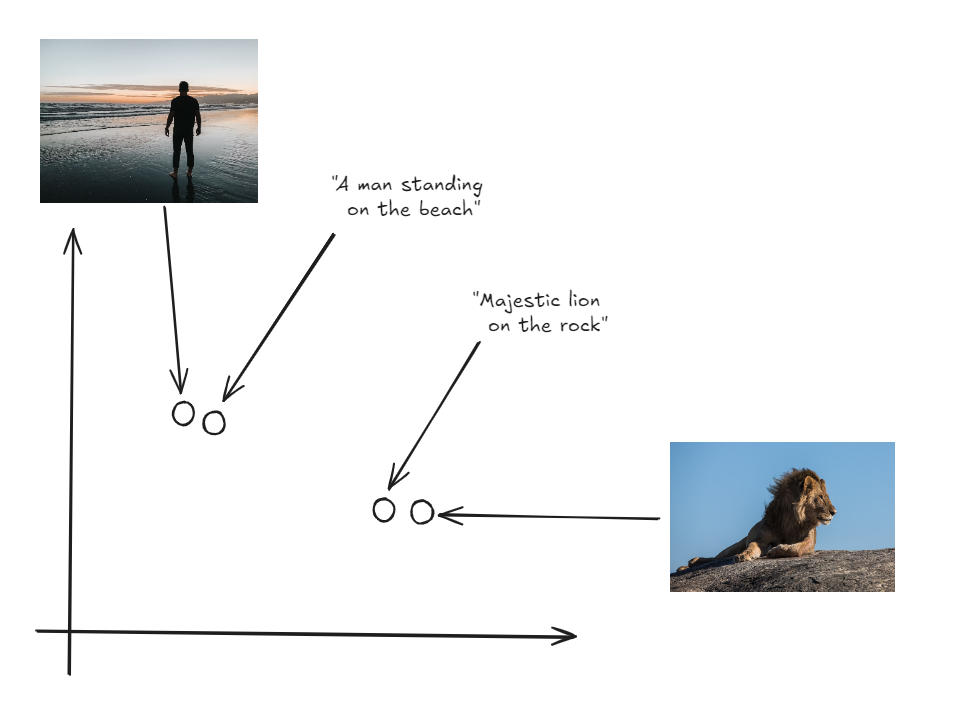
Both Images and labels in the same vector space
To perform zero-shot classification, CLIP first generates embeddings for a set of text descriptions that correspond to different classes (e.g., “a photo of a cat,” “a photo of a dog”). It then generates an embedding for the input image. The model calculates the cosine similarity between the image embedding and each of the text embeddings. Cosine similarity measures the cosine of the angle between two vectors, indicating how closely they align. The text description with the highest cosine similarity to the image embedding is selected as the predicted label. This process allows CLIP to classify images into categories it has never explicitly seen during training, relying solely on the semantic information captured in the text descriptions.
Note: The same approach can applied to build anImage Search Application using CLIP (opens new window).
# Practical Example
Now, when we tested the CLIP model on the Imagenette dataset for zero-shot classification, it performed exceptionally well, achieving over 99% accuracy. This result shows that CLIP can match or even surpass the performance of traditional image classification models.
With such impressive results, it’s clear that CLIP offers a powerful alternative for image classification tasks. Now, let’s dive deeper into how we can implement this model in a practical scenario.
Note: You can find the complete notebook on Github (opens new window).
# Installing Required Libraries
First, we need to install the necessary libraries. Use the following command to install the required packages:
pip install datasets transformers
The datasets library from Hugging Face gives you access to a huge variety of ready-to-use datasets that are super helpful for machine learning projects.
The transformers library, also by Hugging Face, is your go-to for using powerful pre-trained models. In our case, we'll use it to load and work with the CLIP model.
# Importing Dependencies
After the libraries are installed, we can import the required dependencies. These include essential modules for handling data, working with the CLIP model, and visualizing results.
import torch
import numpy as np
from datasets import load_dataset
from tqdm.auto import tqdm
from transformers import AutoProcessor, CLIPModel, AutoTokenizer
from sklearn.metrics import accuracy_score
import matplotlib.pyplot as plt
import seaborn as sns
We'll be using matplotlib and seaborn to create and display visualizations, which will help us better interpret and present our data throughout this project.
# Loading the CLIP Model
To perform zero-shot classification, we load the CLIP model. The model will be loaded onto the GPU if available, otherwise, it will fall back to the CPU. We also load the associated processor and tokenizer.
device = "cuda" if torch.cuda.is_available() else "cpu"
model = CLIPModel.from_pretrained("openai/clip-vit-large-patch14").to(device)
processor = AutoProcessor.from_pretrained("openai/clip-vit-large-patch14")
tokenizer = AutoTokenizer.from_pretrained("openai/clip-vit-large-patch14")
The AutoProcessor is responsible for processing both image and text data so that they are compatible with the CLIP model. The AutoTokenizer converts text into a format that can be understood by the model, generating the necessary tokens for further processing.
Note: For this blog, we are utilizing the free GPU available in Google Colab, which significantly speeds up the processing time.
# Loading the Imagenette Dataset
We proceed by loading the Imagenette dataset, which is a smaller subset of the larger ImageNet dataset. This subset contains 10 classes, making it more manageable for rapid experimentation:
imagenette = load_dataset(
    'frgfm/imagenette',
    '320px',
    split='validation',
    revision="4d512db"
)
The load_dataset function from Hugging Face’s datasets library is used to download and prepare the Imagenette dataset. This version of the dataset consists of images resized to 320 pixels and is split into a validation set to evaluate the model's performance.
# Analyze the Dataset
We start by printing the class labels present in the dataset to understand what categories we are working with:
labels = imagenette.features["label"].names
print(f"Class labels in dataset: {labels}")
The above code will print the following result:
Class labels in dataset: ['tench', 'English springer', 'cassette player', 'chain saw', 'church', 'French horn', 'garbage truck', 'gas pump', 'golf ball', 'parachute']
# Visualizing Class Distribution
To better understand the distribution of images across different classes, we create a bar plot.
plt.figure(figsize=(10, 6))
sns.barplot(x=labels, y=class_counts, palette='viridis')
plt.xticks(rotation=45, ha='right')
plt.title('Class Distribution in Imagenette Dataset')
plt.xlabel('Class Labels')
plt.ylabel('Number of Images')
plt.show()
The above code will generate a bar plot like this: The graph shows that the class distribution in the Imagenette dataset is uneven. However, this imbalance isn't an issue for us since we're not using the dataset for training, but rather for zero-shot classification.
# Selecting and Processing Images
We then iterate through the dataset to select images and their corresponding labels. This step prepares the data for the subsequent embedding generation.
selected_images = []
selected_labels = []

for example in tqdm(imagenette):
    label = example["label"]
    selected_images.append(example["image"])
    selected_labels.append(label)
# Preparing Text Inputs
For zero-shot classification, we convert the class labels into text inputs using the tokenizer. These inputs are fed into the model to generate text embeddings.
text_inputs = tokenizer([f"a photo of a {c}" for c in labels], return_tensors="pt", padding=True).to(device)
The reason for formatting the strings as "a photo of a {label}" is that the CLIP model was trained on similar text-image pairs. This phrasing helps the model better match the text to the corresponding images.
# Generating Text Embeddings
Using the CLIP model, we generate text embeddings for each class label. These embeddings will later be compared with image embeddings to classify the images.
with torch.no_grad():
    label_emb = model.get_text_features(input_ids=text_inputs['input_ids'], attention_mask=text_inputs['attention_mask'])
    label_emb = label_emb.cpu().numpy()
# Batch Processing and Image Embedding Generation
We process the selected images in batches to generate image embeddings. These embeddings are then compared with the text embeddings to calculate similarity scores.
preds = []
batch_size = 50

for i in tqdm(range(0, len(selected_images), batch_size)):
    i_end = min(i + batch_size, len(selected_images))
    images = processor(
        images=selected_images[i:i_end],
        return_tensors='pt'
    )['pixel_values'].to(device)

    with torch.no_grad():
        img_emb = model.get_image_features(images)
        img_emb = img_emb.cpu().numpy()

    # Calculate similarity scores between image embeddings and text embeddings
    scores = np.dot(img_emb, label_emb.T)
    preds.extend(np.argmax(scores, axis=1))
Now, we've got a set of predicted labels for our selected images. Next, we'll explore how well the model performed and the insights these predictions offer.
# Calculating and Displaying Accuracy
Finally, we calculate the zero-shot classification accuracy by comparing the predicted labels with the actual labels.
accuracy = accuracy_score(selected_labels, preds)
print(f"Zero-shot classification accuracy on Imagenette: {accuracy * 100:.2f}%")
The above snippet will give us the following output:
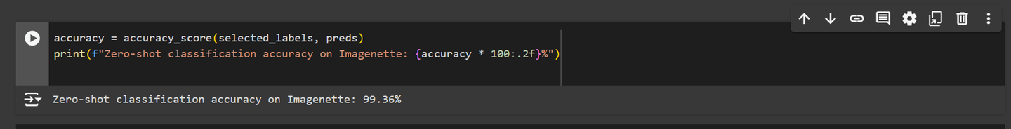
As we can see, the CLIP model performed really well on the Imagenette dataset, achieving high accuracy. This strong performance is due to the high-quality images and the relatively small number of classes in the dataset, making it easier for the model to align the images with their corresponding text descriptions. CLIP was trained on a vast dataset of 400 million image-text pairs, typically using images resized to around 224x224 pixels, which helped it learn to generalize across a wide range of visual and textual data.
However, when lower-resolution images or datasets with more classes are used, the model's performance varies. For instance, when we tested the model on CIFAR-10 dataset, with 32x32 pixel images, the accuracy dropped to 94.76%. Similarly, testing on the SaulLu/Caltech-101 dataset with 102 classes showed lower accuracy 81.21% due to the higher number of classes and varied image quality.
Note: Here you can find the complete notebooks with results for SaulLu/Caltech-101 (opens new window), and CIFAR-10 (opens new window).

Despite these challenges, CLIP remains an excellent choice, particularly when you have limited or no labeled training data. Its ability to perform zero-shot classification and handle various tasks without extensive retraining makes it a valuable tool in situations where traditional models might fall short.