While text searches are pretty common, there are often scenarios where we need to search for images using an image (opens new window) itself as a search query—think of finding similar photos or identifying products from a picture. This approach, known as image-based search (opens new window) or reverse image search, has a lot of applications—online shopping where you snap a photo of something you like to find where to buy it, identification of unknown plants or landmarks, and so on. It's a fascinating field that's becoming more relevant as our visual data grows.
Obviously, it's challenging because we don't have a direct text query to match with. Instead, we need a way to represent images in a form that can be compared effectively. This is where embeddings (opens new window) come into play. By converting images into numerical vectors in a high-dimensional space, embeddings allow us to measure the similarity between images based on their features.
In this blog, we'll go through some of these methods. We'll explore how embedding models are used in image search, examine the algorithms behind them, and see how they make finding similar images possible. Whether you're a developer looking to implement image search or just curious about how it works, this post will shed some light on the topic.
# Classical Methods
In the deep learning (opens new window) era, the concept of finding similar image features in search engines actually predates the widespread adoption of deep learning techniques. As early as 2009, Google Images incorporated a similar image feature (opens new window), and shortly afterwards, content-based image retrieval (CBIR) (opens new window) systems were introduced. This raises a natural question: what were the methods that enabled these image searches without relying on state-of-the-art deep learning models?
# SIFT
The Scale-Invariant Feature Transform (SIFT) (opens new window) was once a highly efficient and go-to algorithm before the advent of deep learning architectures. SIFT identifies key points of interest in an image that are invariant to scaling, rotation, and even some degree of affine distortion and illumination changes. After detecting these key points, SIFT computes feature descriptors by analyzing the local gradient information around each point. These descriptors are typically 128-dimensional vectors that effectively capture the local structure of an image. They can be used as embeddings in various applications, including image matching and retrieval.
SIFT isn’t short of its share of criticism either. It has low efficiency for smaller images, uses a lot of memory (imagine 128-dim vectors for thousands of key points) and is sensitive to illumination. Plus, it was patented as recently as 2020, and as a result, it didn’t get as popular with the community as the other methods.
# SURF
Addressing some of the computational complexity criticisms of SIFT, Speeded-Up Robust Features (SURF) (opens new window) was introduced as a faster alternative. SURF trades a bit of performance accuracy for computational speed. While SIFT relies on first-order image derivatives (gradients) for feature detection and description, SURF uses an approximation of second-order derivatives (Hessian matrix) for faster computation. The feature descriptors generated by SURF are usually 64-dimensional vectors, or 128-dimensional for the extended version, making them suitable for embedding representations in image retrieval tasks.
In addition to these, there are other methods like Histogram of Oriented Gradients (HOG), Oriented FAST and Rotated BRIEF (ORB), and more.
# Implementation
Both SIFT and SURF are easy to implement using the OpenCV (opens new window) package. OpenCV (4.4.0 onwards) has a ready-to-use SIFT_create() function to initialize the sift objects. These objects can be then further used to detect and compute the key points along with their descriptors (embedding vectors).
import cv

image = cv2.imread('AdventureKKH/15.jpg')
grayScaleImage = cv2.cvtColor(image, cv2.COLOR_BGR2GRAY)

sift = cv2.SIFT_create()
keypoints, descriptors = sift.detectAndCompute(grayScaleImage, None)
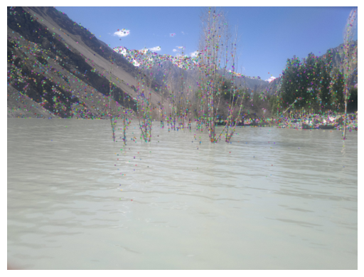
An image can have a lot of key points. Once found, we can simply draw them.
import matplotlib.pyplot as plt

image_with_keypoints = cv2.drawKeypoints(image, keypoints, None)
plt.imshow(cv2.cvtColor(image_with_keypoints, cv2.COLOR_BGR2RGB))
plt.axis('off')
plt.show()

As you can see, these key points are in a big number (6433 precisely), but due to the low contrast with the image, most of them can’t be able to identify. As a better alternative, we can set the flags=cv2.DRAW_MATCHES_FLAGS_DRAW_RICH_KEYPOINTS to visualize them in a little better way.

The features (descriptors) can be visualized in a better way too, using the DataFrame. As you can see, we have a row for every SIFT point (keypoints) and every point’s feature is 128-dimensional.

Since SURF is a patented algorithm, so it’s not allowed to be used directly from the OpenCV. Now, let’s focus on the more common ones, deep architecture-based models.
# Deep Architectures-Based Embeddings
Building on traditional methods like SIFT and SURF, which focus on extracting local features from images, deep learning models offer a more powerful approach to image representation. These models learn hierarchical features (opens new window) directly from data, capturing intricate patterns and structures that are not easily identified by handcrafted algorithms. This advancement allows for more robust and discriminative embeddings, enhancing tasks like image search and retrieval.
There are several ready-to-use (pre-trained) models, such as VGG (opens new window), ResNets (opens new window), Inception (opens new window), MobileNet (opens new window), and others. These convolutional neural networks (CNNs) have been trained on large datasets like ImageNet, enabling them to extract rich and diverse features from images. Unlike traditional algorithms, deep learning models can capture both low-level features (like edges and textures) and high-level concepts (like objects and scenes).

Using these models to calculate embeddings is relatively straightforward. We take a pre-trained model, instead of using the output from the final classification layer, and extract the output from an earlier layer—typically the one just before the classification layer. (opens new window) This output is a high-dimensional feature vector that serves as an embedding, effectively representing the image in a numerical form suitable for similarity comparisons.
For example, let's use ResNet-50, a popular deep-learning model known for its residual connections that help train deeper networks effectively. By removing its last layer, we can obtain embeddings for a given image:
import torch
import torchvision.models as models

model = models.resnet50(pretrained=True)
model = torch.nn.Sequential(*(list(model.children())[:-1]))

with torch.no_grad():
    embedding = model(image.unsqueeze(0))
# ViT based Embeddings
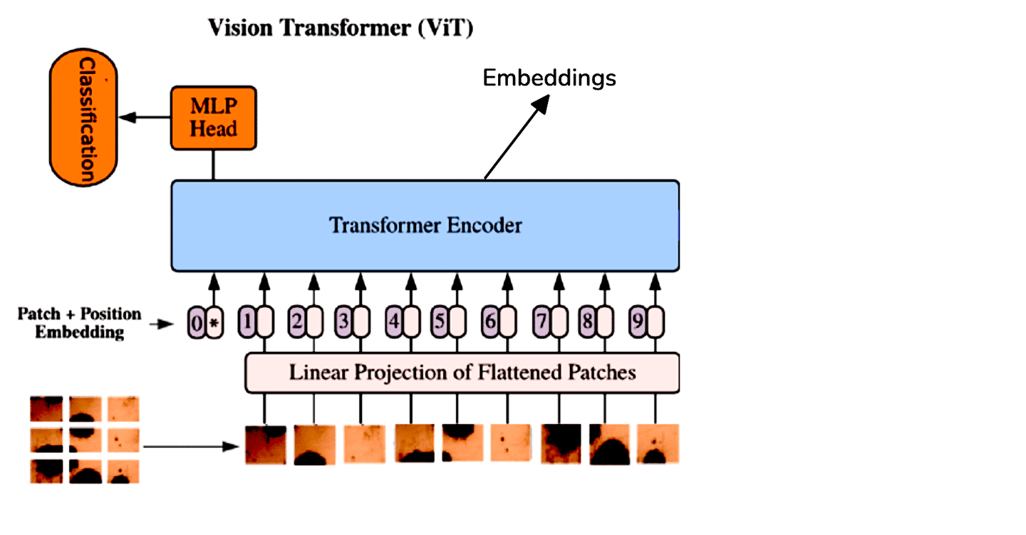
While CNNs have been the standard for image processing tasks, Vision Transformers (ViT) offer a different approach by applying the transformer architecture to image data. ViT treats an image as a sequence of patches and processes it similarly to how transformers handle sequences in natural language processing. This method allows the model to capture global relationships within the image more effectively.
Due to the architectural differences between ViTs and CNNs, we extract embeddings from ViTs by averaging the output tokens from the transformer encoder. For convenience, we can use pre-trained ViT models available through Hugging Face:
from transformers import ViTModel, ViTFeatureExtractor
import torch

model = ViTModel.from_pretrained('google/vit-base-patch16-224-in21k')
feature_extractor = ViTFeatureExtractor.from_pretrained('google/vit-base-patch16-224-in21k')

image = Image.open('AdventureKKH/15.jpg')
inputs = feature_extractor(images=image, return_tensors="pt")

with torch.no_grad():
    outputs = model(**inputs)
    embedding = outputs.last_hidden_state.mean(dim=1)


print(embedding)
Since we are using the default ViT architecture (one used in the original paper [1]), embeddings vector will have 768 dimensions, as we can see here. If you want a better resolution, you can switch to ViT-Large or ViT-Huge (1024 and 1280 lengths respectively).

# Fine-tuning
When working with specialized image types that require model fine-tuning, whether using a Convolutional Neural Network (CNN) or Vision Transformer (ViT), it is often beneficial to freeze all but the final layer of the model. This approach allows for the fine-tuning of the last layer without altering the learned features of the preceding layers.
After the fine-tuning process is complete, the last layer can be removed, similar to previous procedures. With the modified model, images can then be passed through the forward pass to generate the desired embeddings. This method ensures that the model retains its foundational understanding while adapting to the nuances of the specific image data.
# Self-supervised Methods
Just check your own pictures folder and start annotating it. You will clearly get tired after 50 or 100. Fine-tuning requires a lot of labeled data, which is unfortunately neither readily available nor is worthy of spending time on. So a better solution is to use self-supervised learning. There are a number of self-supervised learning methods available, like:
Both SimCLR and MoCo produce two copies of the input image and their embeddings. Then underlying architecture (usually a ResNet) is trained to ensure the contrastive loss is minimized.
CLIP on the other hand uses both image and its textual description embeddings respectively to train the model. This method has become famous as we are seeing a number of similar methods since then. Examples include BEiT (BErt pre-training of image Transformers), VisualBERT and ViLBERT.
Note: To learn more about CLIP, you can read our blog on Zero-shot Classification with CLIP (opens new window).
Here, we will use Moco (v2) to calculate image embeddings.
import torch
import torch.nn as nn
from torchvision import models

class MoCoResNet(nn.Module):
    def __init__(self, base_encoder=models.resnet50, feature_dim=128):
        super(MoCoResNet, self).__init__()
        self.encoder_q = base_encoder(pretrained=False)
        self.encoder_q.fc = nn.Identity()  # Removing final layer

    def forward(self, x):
        return self.encoder_q(x)

model = MoCoResNet()

checkpoint = torch.load('/Users/talha/Downloads/moco_v2_800ep_pretrain.tar', map_location='mps', weights_only=True)
model.load_state_dict(checkpoint['state_dict'])
Image embeddings can be calculated just like we did earlier for the pre-trained normal CNN models.
with torch.no_grad():
    embedding = model(image.unsqueeze(0))
It also returns a 2048-dimensional vector, as we can confirm.

# Applications
These image embeddings can be quite helpful in some image search applications. For example:
- E-commerce: As we already mentioned, it can be quite helpful in online shopping. It can be used in a number of ways. And its one of the number of uses of CBIR.
- Image classification: We can use these embeddings to train CNNs and ViTs too.
- Image captioning: If we use text embeddings too, we can make an image captioning system. CLIP is a very good example.
# Comparison
It would be good to provide a comparative analysis of all the respective models.
| Algorithm | Speed | Strengths | Weaknesses |
|---|---|---|---|
| SIFT | Moderate | Can operate on lesser amount of data | Not scalable, slower for a non-DL method |
| SURF | Fast | Faster | Not as robust as other methods |
| Pre-trained CNNs | Fast | A number of models to choose from, robust | too generic |
| Pre-trained ViTs | Moderate to Fast | Robust | not any significant |
| Fine-tuned Models | Slow (inference is fast, but training can take a lot of time) | Can adapt better to the target data, can give best results | Requires a lot of annotated images and training resources |
| Self-supervised Models | Depends on the training set but usually slow | Doesn’t require annotated images, gives quite good results | Training resources required |
# Conclusion
Embedding methods have transformed image search, enabling us to locate visuals with unprecedented speed and precision. From classical methods like SIFT and SURF to modern deep learning architectures, the evolution of image embeddings has made this transformation possible.
The future of image embeddings looks even more exciting, with trends like multimodal embeddings (opens new window) (combining text, image, and audio data) and self-supervised methods that eliminate the dependency on large labeled datasets. With databases like MyScale (opens new window), which combines SQL and vector search, it's now easier than ever to build advanced image search (opens new window) applications. MyScale supports powerful image embeddings and fast retrieval through vector indexes, providing a solid foundation for future innovations in image search.
As research progresses, we are likely to see even faster, more accurate, and smarter image search capabilities. These advancements will not only enhance user experiences across platforms but also redefine the way we interact with visual information online—making image search as natural and efficient as text search.


